SM 5 BSZ - Computer Design of Very High Gain Yagi Antennas
(April 4 1997)
Published in UKW-Berichte, 4 1996, p 217 - 232. (In German)

Computer Design of Very High Gain Yagi Antennas

SM 5 BSZ, Leif Åsbrink

1. INTRODUCTION

For quite some time modelling of antennas in the computer has been a standard procedure, available to a large number of radio amateurs. Computer programs that automatically optimises antennas are also available and frequently used by amateurs.

Still the design of the optimum antenna for a particular situation is by no means simple. One of the problems is that currently available optimisation programs are not convergent, the optimum antenna that the computer finally finds, depends on the initial antenna from which the optimisation started.

In this article a more convergent method is presented. When applied to long yagis, or arrays of long yagis, this method is fully convergent.

Of course the optimum antenna depends on the intended use. The optimum transmit antenna is usually the one that would give maximum radiation in a certain direction, which is the antenna of maximum gain.

In some cases however the optimum transmit antenna may be the antenna that allows most power in some directions without BCI and TVI.

For the receiver we want maximum S/N. The signal S is proportional to the gain, but lowering the noise N may be much more useful than increasing S. The noise may be thermal due to ohmic losses, or may come from spurious lobes pointing at noise sources.

With the method presented here it is possible to find the optimum antenna for a wide variety of situations.

Since the early sixties my favourite band has been 144MHz. This band is a special case in a rural area where man made noise is practically absent: Ground, sky and antenna have the same temperature, while the receiver noise temperature easily is made much lower.

The optimum antenna both for receive and transmit is then the one with maximum gain.

The yagi producing maximum gain for a given number of elements is certainly not only of theoretical interest, it is the practical solution of my problem: How to make a competitive EME station with a limited antenna size.

2. YAGI MODEL

In 1967 Roger F Harrington published an article "Matrix Methods for Field Problems" [1]. A few years later computer programs based on Harringtons method became available, and I have been using the program that was listed by D. C. Kuo and B. J. Strait [2].

This program is quite general, it can treat arbitrarily bent wires, so the speed is limited and the input it needs is a bit complicated. The program is a faster version of earlier programs [3],[4].

To simplify things, and to save computer time I have modified the program to only accept geomerties made up from arrays of yagi antennas.

I am not aware of any other type of geometry that can compete with the excellent performance of this class of antennas.

Although the rest of this article is about yagi antennas, the generalisation to any antenna type is obvious and I will not give any further comments on that.

The way of operation of the model is in short as follows: All the elements that make up the total antenna system are thought of as being divided into a number of short subsections or segments connected together. For each such segment it is assumed that the current varies linearly from end to end. This leads to triangular expansion functions for the current that allow calculation of a generalised impedance matrix. Using the impedance matrix it is possible to calculate the current in each segment when applying a voltage at the centre of the radiator. From the currents feed point impedance, radiation pattern and ohmic losses are calculated.

A simplified method was published by W2PV [5]. This method is very fast, because only one segment is used for each element. Although not explicitly stated, the current distribution is assumed to be the same on all elements which allows the impedances to be fetched from tables.

If the computer modelling of antennas is unclear, start by reading the article by W2PV.

3. MODEL CALIBRATION.

Obviously the result of a model calculation using the program by Kuo and Strait will depend on the number of expansion functions used for each element. A very critical antenna, the optimised 6 element yagi by Chen and Cheng [6], can be used as an illustration, table 1.


         Number of       Gain                 Impedance
         functions       (dBd)              (Ohms Re, Im)
             3            9.500            31.914    -29.833
             5           10.687            22.834    -16.526
             7           11.272            15.946     -4.913
             9           11.486            12.770      3.575
            11           11.491            11.243      9.669
            13           11.390            10.461     14.212

         Table 1. Gain and impedance for the Chen and Cheng
         6 element yagi calculated with 3 to 13 triangular
         expansion functions for the current on each element.
         All segments of one element were made equal.

From table 1 it seems like it would be necessary to use something like 21 expansion functions for each element to have an acceptable accuracy. Even with a pentium processor this would not be practical even for moderately sized EME antennas because of long computing times. The error caused by using too few expansion functions can be compensated by a correction of the element length, and after some experimenting I have found the following correction factor

1 + .766 / [(M+1)(M+2)] - [ 3.744 - 6.24 / SQRT(M) ]*R/l

Where M is the number of expansion functions for the current on each element, SQRT(M) is the square root of M and R/l is the element radius in wavelengths. When all element lengths are multiplied by this factor prior to the calculation with the Kuo and Strait program the results of table 2 are obtained


          Number of       Gain              Impedance
          functions       (dBd)            (Ohms Re, Im)
              3          11.501           10.972     6.398
              5          11.504           11.418     7.496
              7          11.506           11.655     7.573
              9          11.505           11.653     8.061
             11          11.501           11.547     8.776
             13          11.494           11.407     9.575
          Table 2. Same as table 1, but the element lengths
          are multiplied by a correction factor prior to
          computer modelling.


Table 2 shows that most of the error introduced by having too few expansion functions can be removed by a simple correction factor.

Since all elements have similar lengths an additive correction would produce similar results but it seems more natural to use a multiplicative correction since the effect of too few segments should be smaller for shorter elements where the segments are smaller.

One more correction is needed for each element of a yagi antenna. This is empirically found [7] and means that all element lengths produced by the theory are too long by one and the same amount, depending on element thickness. My explanation for this "end effect correction" is that the theory assumes that the current at the element tip is zero, which is not exactly true.

Some current flows from the cylindrical element surface to the planar element end surface, and further into the air through the small capacitance to infinity from the element tip.

The elements of the model have to be shortened by a small quantity to compensate.

A first guess on how much to remove is that the removed part should have roughly the same area, and therefore capacitance to infinity as the flat end surface.

There may be more reasons for an empirical correction to the element lengths. There are approximations in the method, and they may cause errors that can be absorbed by this type of corrections.

The important thing to know is that when the appropriate corrections are done, the model gives very good agreement with experimental radiation patterns and impedance values even for long yagi antennas with very high Q.

4. GAIN OPTIMISATION

With the gain optimised yagi, vhf amateurs would normally refer to the yagi of a certain boom length that has more gain than all other yagis on the same or shorter booms.

It turns out that this problem is well solved by the simpler problem: For a given element diameter, find the yagi with N elements that gives more gain than any other design.

If the model is used to calculate the gain figure, and then the element lengths and positions of the initial antenna are varied until no more improvement is possible using one or other of the numerical methods available for this kind of problem, it turns out that the final antenna depends on the initial antenna.

It is believed for example in [8] that the reason is that the gain hypersurface has multiple maxima, and that therefore it is impossible to know if a particular maximum is the best possible one.

My opinion is different: The reason for the difficulties is simply that the gain hypersurface is too flat, so the methods previously used are not able to find the extremely small slope towards the global maximum.

With enough numerical accuracy and computing time the maximum gain antenna would be found using traditional methods, but stopping when the improvement is 0.1dB for each iteration as in [8] is certainly not enough.

In the computer program the gain is calculated by numerical integration of the radiation pattern. The integral gives the average over all directions of the radiated power density.

The directivity is then the power density in the forward direction divided by the average power density.

The gain finally is the efficiency multiplied by the directivity.

The efficiency h, is radiated power divided by the sum of radiated power and power converted to heat by ohmic losses.

The key to a convergent optimisation method is to operate on the radiation pattern rather than the gain figure.

The optimisation program uses the antenna calculation package as a subprogram CALC.

The input to CALC is:
N = Number of elements.
D = Element diameter (the same for all elements).
Pi for i between 1 and 2N-1
P1=Length of element 1,
P2=Length of element 2, ...,
PN=Length of element N,
PN+1=coordinate of element 2,
PN+2=coordinate of element 3, ...,
P2N-1=coordinate of element N.
K = number of identical yagis to stack
Xj, Yj, for j between 1 and K is the stacking configuration.

The output of CALC is the radiation pattern in steps of i.e. 2 degrees. The radiation pattern could be a two dimensional array of size i.e. 90*180 containing 16200 complex numbers, each of which represents the electrical field strength in a certain direction.

To get to the gain all these numbers have to be squared, weighted and summed to get the average power density. The forward power density is then divided by this value and finally the result is multiplied by the efficiency.

This process takes quite some time, but it is possible to gain a lot of speed by changing the order of operations.

The radiation pattern of an array of yagi antennas can very closely be approximated as the radiation pattern of a half wave dipole, multiplied by the H pattern of the yagi, multiplied by the radiation pattern that would arise when isotropic radiators were stacked in the stacking configuration.

The optimisation procedure means using the CALC routine many times with different sets of parameters Pi. The changes in P only affects the H pattern of the yagi. Everything else can be calculated once and for all and stored as a weight function, Wk.

The H pattern, Hk is an array of say 90 complex values for 0 to 180 degrees in 2 degree steps. The gain formula then becomes:

G = h * H0*H0 / Sum( Wk*Hk*Hk) . . . . . . . ( 1 )
Sum means summation for k corresponding to 0 to 180 degrees.

Which may be rewritten as:

G = 1 / Sum( Bk * Bk) . . . . . . . . . . . . . . . . .( 2 )
where Bk = (Hk / H0) * SQRT( Wk / h ) . . . ( 3 )

The problem of finding maximum gain is now converted to find the minimum of the sum of squares for the numbers in the array B.

The CALC sub program is rewritten to give B as an output with the parameters P as input. Everything else is held constant.

The problem now has a form that is very well known. It is the "Non-linear Least-squares Fit", fit B to zero in a least squares sense.

If you read about this problem in mathematical textbooks you will find it has a bad reputation: You may find a minimum - but in general it is not possible to be sure that no better minima exist. This is exactly the problem which the yagi optimisation procedures are known for !!

The yagi least squares problem however is a special case. In my experience it will give only a few minima regardless of the initial design. It is easy to find all these minima and select the best one.

5. THE NON - LINEAR LEAST - SQUARES PROBLEM

If you are not interested in mathematics, skip this section.

A comparison of different methods has been published by the US Department of Industry, National Physical Laboratory [9]. Fortran programs are available in the NPL Algorithms Library.

The method I have been using is straight forward. I do not know how it compares to other methods in terms of computational speed and ability to find minima of ill conditioned problems, but I suspect my method is not particularly good.

The least-squares problem is:

Find a point x+ which minimises F(x):

F(x) = Sum( fi(x)*fi(x) ) ,summation for i=1 to m
where x is an array of dimension n, and m>n.

x describes the antenna, and it is the parameter P that gives element lengths and positions. For the N element yagi problem n = 2N - 1.

F(x) = 1 / gain(x)
The x that gives minimum of F(x) will give maximum gain.

fi(x) is B as described in formula (2), the normalised electric far field multiplied by a weight function. The real parts and the imaginary parts of B correspond to different values of i. Calculating B in 2 degree steps from 1 to 179 degrees gives 89 complex values corresponding to i=1 to 178.

By making small steps in x, stepping one element dimension xk at a time, the corresponding change in the m points of the far field is obtained from a new calculation of F(x). This is an inefficient, but simple way of getting J(x), the m * n Jacobian matrix of f(x) whose ith row is

Dfi(x) = ( dfi/dx1, dfi/dx2, ... ,dfi/dxn )

If all fi are linear functions of x, we have the linear least-squares problem, and x+ can be found in one step using standard procedures.

If the linear least-squares subroutine is used to solve the non-linear yagi problem, the solution is far away from the initial antenna, and effects of non-linearity cause the gain to go down in stead of up.

By adding n more rows in J(x):
Dfi+1(x) = ( a,0,0,,,0 ),
Dfi+2(x) = ( 0,a,0,,,0 ),
. . .
Dfi+n(x) = ( 0,0,0,,,a ),
the linear least-squares solution to the new problem becomes a steepest descent improvement to the original yagi problem if a is large enough. By repeating the process while gradually reducing a the non-linear problem may be solved.

To avoid false minima due to numerical difficulties it helps to alternate between a few different ways to calculate J(x). I have been using 4 different ways:

First, J1(x) is calculated with each xj stepped in the positive direction.

Second, J2(x) uses a new set of x variables that are linear combinations of the original x variables. The linear combinations are the eigenvectors of the square matrix J1(x)TJ1(x)

Third, J3(x) is calculated with each xj stepped in the negative direction.

Fourth, J4(x) same as J2(x), but using J3(x)TJ3(x)

It is not necessary to recalculate J(x) for each iteration. By monitoring the non-linearity it is easy to decide when it is time to recalculate.

An appropriate name for this method of optimising yagis is "The brute force method".

The way of getting J(x) from differences of complete calculations is inefficient, but good enough considering the capacity of modern desk top computers. Probably the way of solving the least squares problem is also a good reason for this name.

6. ELEMENT DIAMETERS AND OHMIC LOSSES

The inclusion of ohmic losses in the yagi model is very important, particularly for thin elements. The reason for this is that the gain optimised yagi is a form of superdirective antenna.

Superdirectivity means that the currents in the antenna are very high, and that the radiation from the different parts of the antenna cancels more or less in all directions. Obviously less in the forward direction, and more to the sides, which causes the desired radiation pattern.

The near field is much stronger, since near the antenna there is no cancellation of fields.

A superdirective antenna is sensitive to metal in the near field, and care has to be taken when using highly optimised yagis.

Superdirectivity means that energy is stored in the antenna - which causes the antenna to have a high Q, and a narrow bandwidth.

For equal currents, the magnetic energy stored in a half-wave element becomes higher if the element is made thinner.

The magnetic energy is L*I*I, inductance times current squared, and inductance per length unit is higher for a thinner conductor.

With thin elements the Q becomes higher and the bandwidth lower.

To illustrate the significance of ohmic losses I have optimised a set of 6 element antennas made from an ideal super-conductor. Table 3 shows these antennas with and without ohmic losses.

The antennas optimised without ohmic losses have low impedances and high currents. The convergency of the optimisation process is very slow, and the optimum shallow.


 6 element 144.1MHz yagis optimised for ideal superconducting elements

Diam. Element positions and lengths Gain 1dB bw Impedance (mm) (mm) (dBd) (MHz) Re Im (Ohm) 0.001 0.0 4.5 719.0 1532.2 2381.0 3191.5 11.7799 0.043 0.002 -2.3 1034.9 1033.2 1002.1 993.0 989.5 994.5 -2.85 503 22.8 0.01 0.0 3.5 718.5 1532.5 2380.6 3192.3 11.7800 0.048 0.001 -2.5 1034.8 1033.5 995.4 984.6 980.6 986.3 -2.47 73.6 4.2 0.1 0.0 3.6 714.4 1528.0 2378.1 3188.3 11.7805 0.075 0.001 -0.93 1034.8 1033.4 985.5 972.2 967.1 974.3 -1.33 8.6 -4.0 1 0.0 68.3 744.7 1558.5 2406.5 3216.7 11.7794 1.2 0.26 -16.96 1035.7 1002.4 968.5 951.5 945.2 954.1 9.32 1.05 -16.96 10 0.0 79.7 747.8 1562.9 2411.8 3221.0 11.7804 2.1 0.34 -8.76 1035.9 991.4 933.4 909.2 900.6 913.1 11.04 0.42 -8.76 20 0.0 100.9 758.5 1574.5 2423.2 3231.8 11.7811 3.1 0.52 -7.77 1034.7 975.5 914.0 886.3 876.7 891.0 11.49 0.56 -7.77 60 0.0 113.1 764.8 1582.9 2431.9 3238.3 11.7827 4.9 0.63 -2.90 1034.5 952.3 862.4 826.7 814.9 833.5 11.70 0.64 -2.90 Table 3. Dimensions and performance for 6 element yagis, optimised for max gain without ohmic losses. For each antenna gain and impedance is calculated with and without ohmic losses, upper and lower lines for each entry in the table.


When ohmic losses are neglected, the gain is independent of the element diameters.

Only for diameters above 10 mm these antennas have a reasonable performance when losses are included.

Table 3 shows that it is necessary to include ohmic losses in the optimisation procedure.

In fact I believe that neglecting this is the main reason for convergency problems when optimising yagi antennas.

To calculate the ohmic losses in an approximate way a centre load was placed in each element.

The load impedance in ohms was assumed to be 0. 44 / d, where d is element diameter in mm. The value 0.44 comes from experiments with coaxial resonators, for which I have measured the Q and this is a reasonable approximation for the losses at 144 MHz for aluminium elements with diameters between 5 and 10 mm.

Table 4 shows 6 element antennas, optimised for aluminium elements of different diameters, ohmic losses included during the optimisation process.

From table 4 it is clear that the rule in the ARRL handbook: "Avoid thinner elements than 4 mm" is well founded, and that the much older one in VHF Handbook, Orr, 1956 "In all cases it has been found impossible to secure as high a forward gain figure with thick elements as with thin ones" is not.


   6 element 144.1MHz yagis optimised for aluminium elements

                                                      1dB   Imped.
Diam.       Element  positions and lengths     Gain   BW    (Ohms) Eff.
(mm)                    (mm)                   (dBd)  (MHz) Re/Im   %

 2      0.0  486.2 1024.1 1828.8 2669.0 3459.2 11.43   3.0   8.80  94.02
     1021.7  979.3  959.5  940.3  933.7  943.5               1.46

 4      0.0  448.3  983.6 1786.1 2629.9 3426.6 11.56   3.3   6.71  96.21
     1021.7  965.4  951.2  929.6  921.9  932.5              -5.08

 6      0.0  425.9  960.8 1763.3 2609.1 3408.9 11.62   3.5   5.82  97.14
     1021.7  960.1  945.0  921.8  913.2  924.6              -5.11

 8      0.0  408.7  944.2 1748.8 2594.5 3396.4 11.65   3.6   5.24  97.66
     1021.6  954.2  939.8  915.2  906.3  918.1              -6.30

10      0.0  395.8  933.5 1737.3 2584.4 3387.1 11.67   3.6   4.86  98.01
     1021.5  949.2  935.1  909.6  900.2  912.4              -7.16

20      0.0  352.4  900.2 1706.5 2554.6 3360.0 11.71   4.1   3.79  98.80
     1020.9  928.9  916.3  887.2  876.6  890.5              -10.3

60      0.0  284.4  855.8 1666.8 2515.8 3321.8 11.75   5.5   2.61  99.45
     1020.6  895.9  865.0  828.0  815.1  833.2              -6.79

Table 4.   Dimensions and performance for 6 element yagis, optimised
for max gain with approximate ohmic losses included.


Thin elements give high Q, but it is a misconception that high Q in itself gives high gain. although it is impossible to get high gain from a small antenna without high Q[10].

Thicker than usual elements give slightly more gain on a slightly shorter than usual boom.

This should be noted by those who design yagis for higher bands, where the low sky temperature makes low losses important.

7. COMPARISON WITH EARLIER PUBLISHED RESULTS

The simple and straight forward brute force approach described above was used to try to improve the design by Chen and Cheng[6]. This design was optimised for lossless elements. This antenna was adjusted for 10 mm element diameters [7]. Dimensions for this antenna, for 144.1MHz are given in table 5.

           Element positions (mm):   0  519  1120  1963  2634  3511
           Element lengths (mm):  1007  957   925   910   920  910

           Table 5. Chen and Cheng 6 element yagi adopted for
           144.1MHz and 10mm element diameter


Fig 1. Gain above dipole vs frequency for the 6 element Chen and Cheng design compared with the 6 element optimum antenna produced by the brute force optimisation method. 1 dB gain bandwidth is indicated. Solid lines are with ohmic losses included, and dotted lines are for lossless antennas.


The optimisation was done with and without the inclusion of ohmic losses, and produced the 10 mm antennas of table 3 and table 4.

The theoretical gain as a function of frequency for initial and final antennas are shown in figure 1.

The gain figure presented by Chen and Cheng is 13.356 or 11.26dBd. It is lower than the 11.56dB that I get.

The program by K6STI, YO vers 1.00, gives a gain figure of 11.50 dBd for the 10 mm Chen Cheng design, and I think that the value by Chen and Cheng is too low.

Very probably the difference between the antennas is properly calculated even if there is a small uncertainty about the absolute gain figure.

For lossless antennas, solid lines in fig 1, the gain improvement is 0.22dB with a boom that is 3.22 m compared to 3.51 of the Chen and Cheng design. The improvement in gain per boomlength is 15% or 0.6dB.

When ohmic losses are included, dotted lines in fig 1, the gain improvement is 0.16 dB, and gain per boomlength is improved by 7.5% or 0.3dB.

The reason for a significant improvement over the Chen and Cheng design is that they first optimised the spacings for fixed element lengths, and then optimised the lengths, keeping the spacings that were appropriate for the initial lengths.

Obviously the simultaneous adjustment of lengths and spacings is more flexible and hence more likely to produce the real optimum.


           Initial
             ( G=12.24dBd, reZ=7.6 Ohms, imZ=-15 Ohms, h=97.0% )
          Position  0    0.654 1.099 1.851 2.603 3.138 3.760 4.513
          Length  1.003  0.956 0.948 0.929 0.912 0.866 0.902 0.923

           False optimum, 7elements (0.149 m long can be removed)
             ( G=12.39dBd, reZ=5.8 Ohms, imZ=-21 Ohms, h=96.5% )
          Position  0    0.456 0.983 1.787 2.646 2.730 3.517 4.334
          Length  1.018  0.941 0.944 0.921 0.909 0.149 0.906 0.920

          Long optimum
             ( G=13.06dBd, reZ=5.5 Ohms, imZ=-29 Ohms, h=96.1% )
          Position  0    0.467 0.992 1.797 2.663 3.553 4.442 5.274
          Length  1.018  0.932 0.944 0.920 0.908 0.901 0.901 0.917

          Short optimum
             ( G=12.43dBd, reZ=21 Ohms, imZ=-156 Ohms, h=97.2% )
          Position  0    0.342 0.472 1.026 1.807 2.658 3.527 4.344
          Length  1.018  0.766 0.953 0.939 0.921 0.910 0.907 0.921

          Optimized for 50 Ohms
             ( G=12.42dBd, reZ=50 Ohms, imZ= 0 Ohms, h=97.2% )
          Position  0    0.364 0.487 1.011 1.802 2.658 3.528 4.346
          Length  1.019  0.922 0.953 0.942 0.921 0.910 0.906 0.920

          Nice, near optimum
             ( G=12.39dBd, reZ=50 Ohms, imZ= 0 Ohms, h=98.2% )
          Position  0    0.409 0.702 1.254 2.011 2.849 3.706 4.508
          Length  1.013  0.961 0.958 0.934 0.919 0.909 0.906 0.920


          Table 6. Physical dimensions of the design by Longsomboon
          et al, initial [8] and optimised antennas produced with the
          brute force method with this design as the initial antenna.
          See text for explanation. Dimensions are given in meters
          and the frequency of optimum is 144.5MHz.
          The element diameter is 5.2mm for all elements in table6.


Another optimised antenna was given by Longsomboon, Green and Cashman [8]. For this antenna, using only 5.2 mm elements, I have included the ohmic losses in all calculations. Gain vs frequency is given in fig 2 and physical dimensions in table 6.

When this antenna is used as the initial antenna, the brute force method produces a false optimum, that uses one element less than the initial antenna, fig2 and table 6.

The iterations are stopped when no further improvement is possible, which happens when the unused element is short enough to have no influence.

By removing the very short element, the false optimum 8 element antenna becomes an optimised 7 element yagi. By adding a director at a normal position in front of this 7 element yagi, a new initial antenna is obtained.

Again running the brute force optimisation gives the long optimum antenna of table6 and fig 2. The gain improvement over the design of Longsomboon et al is 0.8dB. This comparison is unfair, since the boom has become much longer.


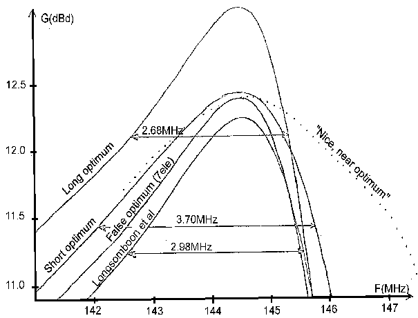
Fig 2. Gain above dipole vs frequency for the 8 element design by Longsomboon, Green and Cashman, compared with 8 element optimum antennas produced by the brute force optimisation method. The intermediate 7 element design is also shown, see text. -1 dB gain bandwidth is indicated.


For long yagis the practical optimum antenna is the best antenna at a certain boom length rather than the antenna using the smallest number of elements.

Anyhow this antenna is the optimum 8 element yagi with element diameter 5.2mm. Slightly more gain can be obtained by increasing element diameter and/or replacing aluminium with copper.

Adding one normal director 0.1 meter in front of the radiator of the false optimum antenna, removing the unused one, forms another initial antenna.

Running the brute force optimisation on that produces the yagi named "short optimum" in table2, and fig 2.

Comparison with the design by Longsomboon et al shows that the gain has increased by 0.19dB (4%), the bandwidth is increased by 25% while the boom length is reduced by 4%.

Attempts to add more elements between the others were not successful, i.e. initial antennas with a 9th element inserted loose one element and come back to the short optimum.

8. CONTROLLING IMPEDANCE AND OTHER PROPERTIES

The optimisation procedure is the simultaneous minimising of several functions of the antenna geometry.

We are free to add more terms into the sum of squares, and with suitable weight factors it is possible to control to what extent these terms contribute to the sum of squares.

Two natural things to add to F(x) are cz*(Re(Z)-50)*(Re(Z)-50) and cz*Im(Z)*Im(Z).

These terms are zero when the feed point impedance is 50 ohms resistive and hence the optimisation now will tend to give 50 ohm antennas.

If 50 ohm feed impedance can be obtained with only a small loss of gain, a very small value on the coefficient cz is required.

Different values of cz will give different compromises between gain and feed point impedance.

In this way the optimised 50 ohms antenna in table2 is obtained. The loss of gain is only 0.01dB, and the frequency response is about 7% narrower.

One more term that I like to add to F(x) is cl*(ohmic losses squared). The reason is that I want a safety margin for degradation of performance due to ohmic losses, from errors in theory and from degraded element surfaces due to ageing.

With the weight factors that I have adopted as my favourites, cz=0.005 and cl=10, the antenna labelled nice, near optimum is obtained as the output of the brute force optimisation.

For the "nice" antenna, the gain is 0.04dB below maximum on a boom that is 4% longer.

These degradations allow a reduction of the losses by 35% and a bandwidth increase of 39%.

If antennas are designed for some other band than 144MHz, it is possible to change the equations to produce max G/T, or whatever other combination of properties the model is able to calculate for any given antenna geometry.

9. GAIN VS BOOM LENGTH FOR YAGI ANTENNAS.

With the "nice" parameters I have made a large number of calculations on different numbers of elements and with different stacking configurations.

In all these calculations I have chosen to make the element diameters 10mm.

The 8 element design gives a gain figure of 12.47dBd on a 4.387m boom.

Fig 3 shows the gain of these antennas, and a set of other ones [11] plotted against the boom length.

The "nice" antennas are about 0.5 dB better than typical EME antennas of 3 to 5 wl boomlength. For very long, or short booms the gain is about 1 dB above the straight line of optimum antennas in [11]. For more than two years I have been using a 4-stack of 14 element cross yagis designed as described above. I am very satisfied with the results, good places in EME contests show that it is possible to get these very high performance antennas to work in the real world.

Great care has to be taken however, and I will come back to that, and to various numerical results, particularly related to stacking, in a second article.

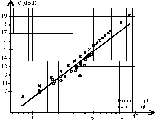
Fig 3. Yagi antenna gain at 144MHz versus boom length. The dots and the straight line are from ref [11], the crosses are the "nice" 50 ohm brute force designs.


References:

1. Roger F Harrington,"Matrix Methods for Field Problems, " Proc. IEEE, Vol 55, No. 2, pp. 136-149; February 1967.

2. D. C. Kuo and B. J. Strait, "Improved programs for analysis of radiation and scattering by configurations of arbitrarily bent thin wires,". Syracuse University, Syracuse, New York. Manuscript.

3. H. H. Chao and B. J. Strait, "Computer programs for radiation and scattering by arbitrary configurations of bent wires," Scientific Report No. 7 on Contract F19628-68-C-0180, AFCRL-70-0374; Sept 1970.

4. D. C. Kuo and B. J. Strait, "A program for computing near fields of thin wire antennas," Scientific report No. 14 on Contract F19628-68-C-0180, AFCRL-71-0463; Sept 1971.

5. James L. Lawson, W2PV, "Yagi antenna design: performance calculations," Ham Radio, Jan 1980, pp. 22-27.

6. C. A. Chen and D. K. Cheng, "Optimum element lengths for Yagi-Uda arrays," IEEE Trans. Antennas Propagat., vol. AP-23, pp. 8 - 15, Jan 1975.

7. L. Asbrink, "The optimum 6 element Yagi-antenna," VHF Communications, vol 14, No 1, Spring 1982.

8. N. Longsomboon, H. E. Green and J. D. Cashman, "Numerical optimisation of Yagi-Uda arrays", Monitor - Proceedings of the IREE Australia, Nov 1977.

9. P. E. Gill and W. Murray, "Algorithms for the solution of the non - linear least - squares problem", NPL Report NAC 71, 1976.

10. R. L. Fante, "Maximum possible gain for an arbitrary ideal antenna with specified quality factor", IEEE Trans. Antennas Propagat., vol. 40, pp. 1586 - 1588, Dec 1992.

11. Rainer Bertelsmeier, DJ9BV, "Gain and Performance Data of 144 MHz Antennas", DUBUS-magazin, no 3, pp 181-189, 1988.

To SM 5 BSZ Main Page
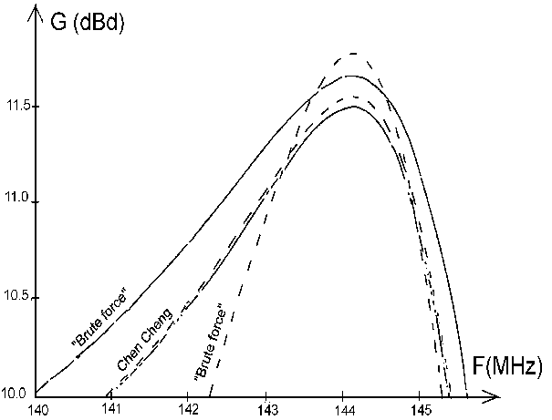